Ridgeline plots to study subnational rainfall patterns in Vietnam
Using {ggridges} and {ggplot2} to create ridgeline plots in R
Overview
Ridgeline plots are a type of chart that displays the distribution of a numeric variable for different categories. These plots are commonly used to visualize changes in distributions over time. To showcase how to create ridgeline plots with {ggplot2} and {ggridges} in R, I will use data on monthly rainfall at some stations by provincies and month in Vietnam, from 2002 to 2024.
Set-up
First, we install and load the necessary R packages.
About the data
Data come from the National Statistics Office of Vietnam and is available at their website. I downloaded the data and saved it in an Excel file called rainfall-vietnam.xlsx.
rainfall_vietnam <- read_excel("rainfall-vietnam.xlsx")Data is not in a tidy format, so I will need to wrangle it.
rainfall_vietnam <- rainfall_vietnam |>
  rename(year = `Monthly rainfall at some stations by Year, Cities, provincies and Month`,
         city = `...2`) |>
  fill(year) |>    # `fill()` replaces missing data from top to bottom
  rename_at(vars(`...3`:`...14`),
            ~ month.name
            ) |> # row 2 contains the name of the months
  slice(-c(1:2)) |> # remove first two rows
  mutate_at(vars(January:December),
           ~ as.numeric(.)) |>
  pivot_longer(cols = January:December,
               names_to = "month",
               values_to = "rainfall")
This information looks like this:
rainfall_vietnam |>
  head(15) |>
  kbl(
    caption = "Monthly rainfall by month in Vietnam, 2002-2024"
    ) |>
kable_paper("hover", full_width = F)| year | city | month | rainfall |
|---|---|---|---|
| 2024 | Lai Chau | January | 185.2 |
| 2024 | Lai Chau | February | 44.5 |
| 2024 | Lai Chau | March | 69.1 |
| 2024 | Lai Chau | April | 27.7 |
| 2024 | Lai Chau | May | 383.9 |
| 2024 | Lai Chau | June | 541.8 |
| 2024 | Lai Chau | July | 395.4 |
| 2024 | Lai Chau | August | 362.6 |
| 2024 | Lai Chau | September | 164.7 |
| 2024 | Lai Chau | October | 148.1 |
| 2024 | Lai Chau | November | 4.4 |
| 2024 | Lai Chau | December | 21.9 |
| 2024 | Son La | January | 55.8 |
| 2024 | Son La | February | NA |
| 2024 | Son La | March | 14.3 |
Creating the ridgeline plots
I will create three versions of the ridgeline plot. First, the ridgeline plot will show the interquantile range of rainfall by month in Ha Noi. Here, the colors represent different quantiles of the distribution of rainfall per month. To show this, I will plot the data from Ha Noi, capital of Vietnam.
rainfall_vietnam <- rainfall_vietnam |>
  mutate(month = factor(month, levels = month.name)) # Important to order months in the correct order

# More font alternatives can be found here https://fonts.google.com/
font_add_google("Oxygen", "Oxygen")

showtext_auto()

rainfall_vietnam |>
  filter(city == "Ha Noi") |>
ggplot(aes(x = rainfall,
           y = reorder(month, desc(month)),
           fill = after_stat(quantile)
           )) +
    stat_density_ridges(quantile_lines = FALSE,
                        geom = "density_ridges_gradient",
                        calc_ecdf = TRUE,
                        color = "black",
                        scale = 1.5) + # Height of ridges
    scale_fill_manual(
      name = "Quantiles",
      values = c("#CCFFFF", "#99EDFF", "#4CC3FF", "#007FFF"),
      labels = c("(0, 0.25]", "(0.25, 0.5]", "(0.5, 0.75]", "(0.75, 1]")
      ) +
  ggtitle("Mean monthly rainfall in Ha Noi, Vietnam | 2002-2024.",
          subtitle = str_wrap("The rainy season in Ha Noi extends from May to early November, peaking in June, July, and August when precipitation is at its highest.", width = 110)
          ) +
  xlab("Monthly rainfall in millimeters") +
  ylab("") +
  labs(caption = "Source: National Statistics Office of Vietnam") +
  theme_minimal(
    base_family = "Oxygen",
    paper = "#EEEEEE"
    ) +
  theme(

    plot.margin = margin(0, 40, 0, 40),

    plot.title = element_text(
      color = "#0D47A1",
      face = "bold",
      size = 100,
      hjust = 0,
      margin = margin(15, 0, 0, 0)
    ),
    plot.title.position = "plot",

    plot.subtitle = element_text(
      color = "#1976D2",
      face = "bold",
      size = 85,
      hjust = 0,
      margin = margin(0, 0, 20, 0),
      lineheight = 0.3
    ),

    axis.title = element_text(
      color = "#0D47A1",
      face = "bold",
      size = 70
    ),
    axis.text = element_text(
      color = "#1976D2",
      face = "bold",
      size = 60
    ),

    plot.caption = element_text(
      color = "#0D47A1",
      face = "bold",
      size = 60,
      hjust = 1,
      margin = margin(25, 0, 5, 0)
    ),

    legend.position = "top",
    legend.title = element_text(
      face = "bold",
      color = "#0D47A1",
      size = 60,
      hjust = 1
    ),
    legend.text = element_text(
      face = "bold",
      color = "#0D47A1",
      size = 60,
      hjust = 1
    ),

  )
# showtext_opts(dpi = 320)
# ggsave(
# "rainfall-vietnam-ridgeline.png",
# dpi = 320,
# width = 15,
# height = 11,
# units = "in"
# )
# showtext_auto(FALSE)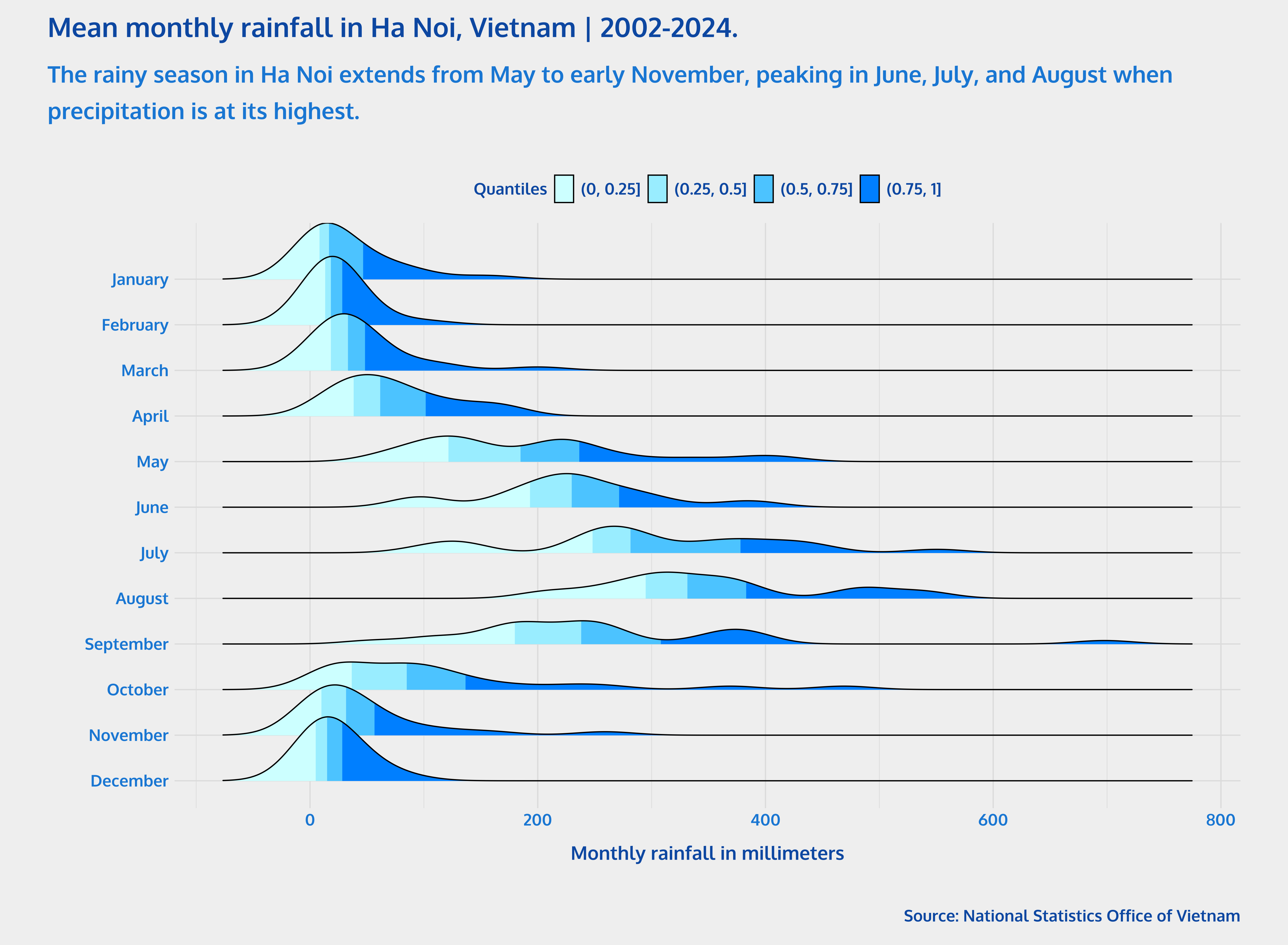
In the second version of the ridgeline plot, I will use a gradient with a continuous fill color scale to represent the amount of rainfall. I will also use other font and color choices. To show this, I will plot the data from Nha Trang, a coastal city and the capital of Khánh Hòa Province.
# More font alternatives can be found here https://fonts.google.com/
font_add_google("Bree Serif", "Bree Serif")

showtext_auto()

rainfall_vietnam |>
  filter(city == "Nha Trang") |>
ggplot(aes(x = rainfall,
           y = reorder(month, desc(month)),
           fill = stat(x)
           )) +
    stat_density_ridges(quantile_lines = FALSE,
                        geom = "density_ridges_gradient",
                        color = "white",
                        scale = 2.8) + # Height of ridges
    scale_fill_distiller(
      direction = 1,
      name = "",
      palette = "RdPu"
      ) +
  ggtitle("Mean monthly rainfall in Nha Trang, Vietnam | 2002-2024.",
          subtitle = str_wrap("The wet season in Nha Trang lasts from September to December.", width = 110)
          ) +
  xlab("Monthly rainfall in millimeters") +
  ylab("") +
  labs(caption = "Source: National Statistics Office of Vietnam") +
  theme_minimal(
    base_family = "Bree Serif",
    paper = "#767F8B"
    ) +
  theme(

    plot.margin = margin(0, 40, 0, 40),

    plot.title = element_text(
      color = "white",
      face = "bold",
      size = 100,
      hjust = 0,
      margin = margin(15, 0, 0, 0)
    ),
    plot.title.position = "plot",

    plot.subtitle = element_text(
      color = "white",
      face = "bold",
      size = 85,
      hjust = 0,
      margin = margin(0, 0, 20, 0),
      lineheight = 0.3
    ),

    axis.title = element_text(
      color = "white",
      face = "bold",
      size = 70
    ),
    axis.text = element_text(
      color = "white",
      face = "bold",
      size = 60
    ),

    plot.caption = element_text(
      color = "white",
      face = "bold",
      size = 60,
      hjust = 1,
      margin = margin(25, 0, 5, 0)
    ),

    legend.position = "bottom",
    legend.title.position = "bottom",
    legend.key.size = unit(1, "cm"),
    legend.title = element_text(
      face = "bold",
      color = "white",
      size = 60,
      hjust = 0.5
    ),
    legend.text = element_text(
      face = "bold",
      color = "white",
      size = 60,
      hjust = 0.5
    ),

  )
# showtext_opts(dpi = 320)
# ggsave(
# "rainfall-vietnam-ridgeline_gradient.png",
# dpi = 320,
# width = 15,
# height = 11,
# units = "in"
# )
# showtext_auto(FALSE)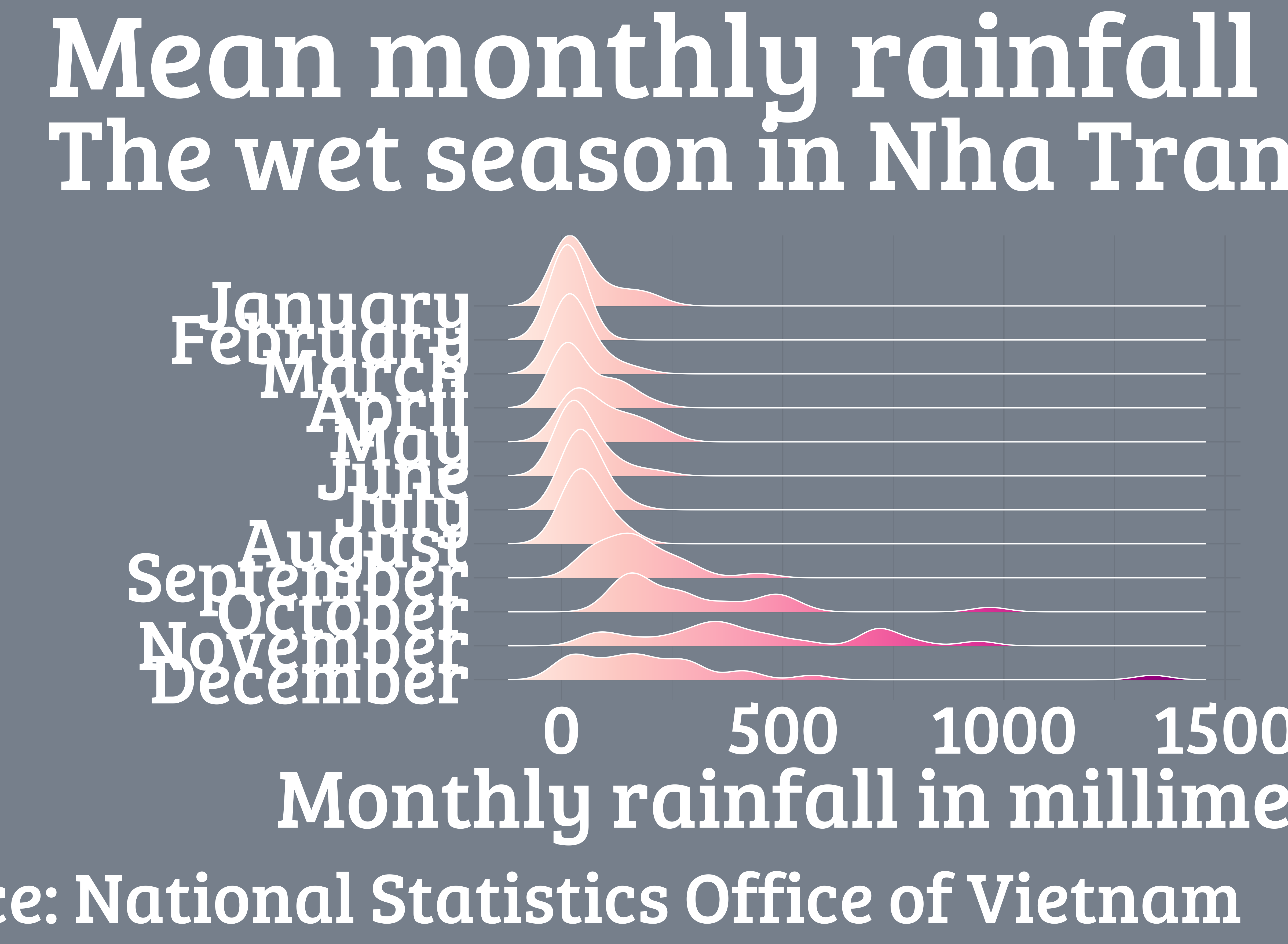
Citation
@online{torres_munguía2025,
  author = {Torres Munguía, Juan Armando},
  title = {Ridgeline Plots to Study Subnational Rainfall Patterns in
    {Vietnam}},
  date = {2025-09-15},
  url = {https://juan-torresmunguia.netlify.app/blog/posts/vietnam-rainfall-ridgeline-plot/},
  langid = {en}
}